Brandon Sandhu

Combining the stochastic oscillator indicator and the moving average indicator to create a trading strategy

Written by Brandon Sandhu on 21/08/2023

Introduction

In this article we shall understand the basics of a specific stochastic indicator and the moving average indicator and combine these two trading indicators to create an unconventional trading strategy using python.

Both of the aforementioned indicators are standard in the classical trading market so to make ourselves stand out, we require new ideas that are both unconventional and not utilised generally. Everyone uses the standard indicators but not many understand how the indicators work on a foundational level and thus we will aim to both understand and extend how these indicators (specifically the ones mentioned above) work.

Our two indicators of concern are the Stochastic Oscillator and the Moving Average Convergence/Divergence (MACD) with the main goal being to remove any false signals.

Stochastic Oscillator

The Stochastic Oscillator is a momentum-based indicator which is used to decide whether a market is in an overbought or oversold state.

An overbought market is one where the prices of stocks have risen very sharply and is expected to decline in value. Often we also describe an overbought market as bullish which means to characterise the stock market with rising stock prices.

An oversold market is (as naturally expected) one where the prices of stocks have fallen very sharply and is expected to rise in value. Often we also describe an oversold market as bearish which means to characterise the stock market with falling stock prices.

The output values of the Stochastic Oscillator always lie in the region 0-100 due to a normalisation function. The generally accepted thresholds for overbought and oversold states are considered to be 70 and 30 respectively but this can vary from trader to trader.

The Stochastic Oscillator has two main components outlined below:

%K Line: The most important component of the Stochastic Oscillator, the purpose of this line is to indicate whether the market is in an overbought or oversold state. It is calculated by subtracting the lowest price the stock has reached over a specified number of periods from the closing price of the stock. Then this difference is divided by the value calculated by subtracting the lowest price the stock has reached over a specified number of periods from the highest price of the stock. The final value is arrived at by taking the computed value from the above steps and multiplying by 100. If we choose the number of periods to be set to 14, then we can compute the %K line by:
%K = 100 * ((14 DAY CLOSING PRICE - 14 DAY LOWEST PRICE) / (14 DAY HIGHEST PRICE - 14 DAY LOWEST PRICE))
%D Line: Is simply the moving average of the %K line for a specified period. It will be a smoother line graph than the %K line.

This is all thats required to calculate the components of the Stochastic Oscillator.

For recall, the Moving Average indicator sums up the data points of a stock over a specified number of periods and divides the total by the number of data points to arrive at an average. It can be considered as a constantly updated averaging indicator.

Let us analyse a graph where Apples closing price data is plotted alongside its Stochastic Oscillator calculated with number of periods as 14 and 3 respectively. This will allow us to understand how to use the indicator.

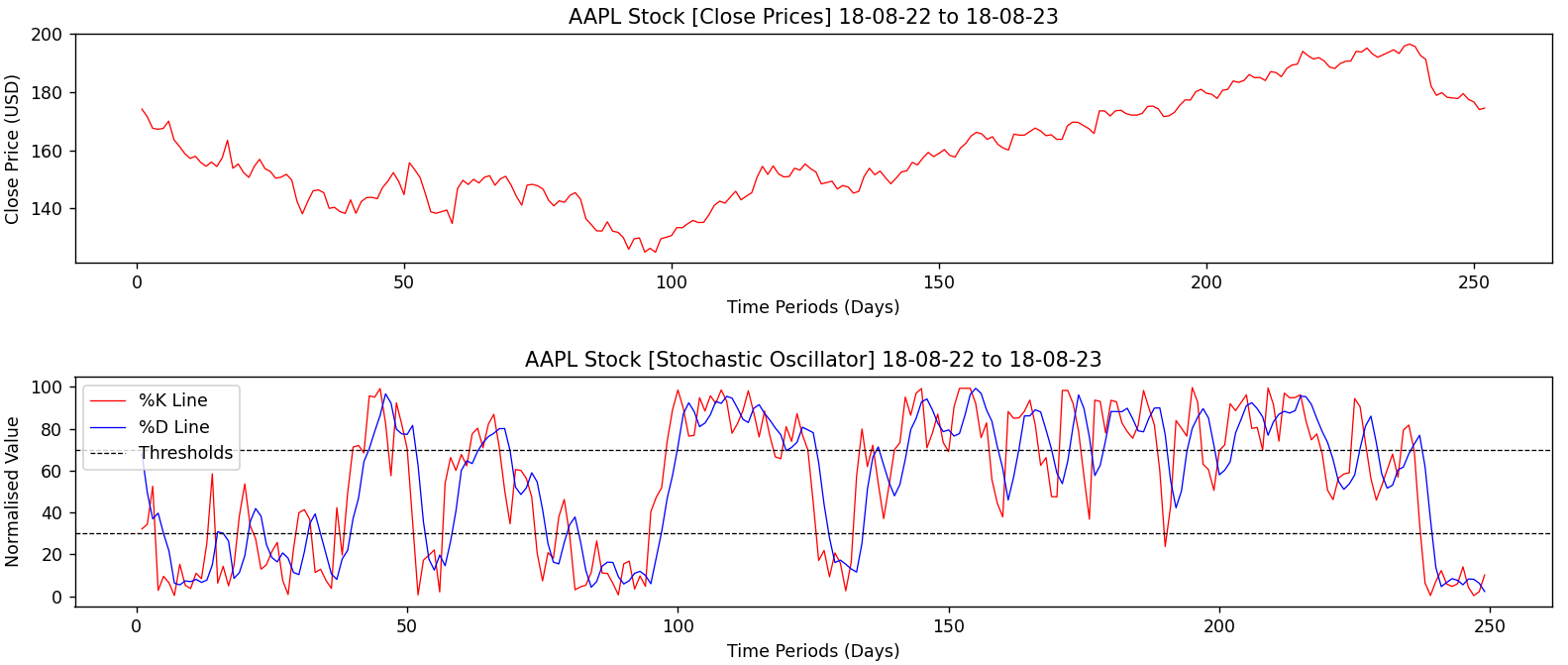
Source: Brandon Sandhu

The panel above consists of two sections: the upper graph represents the line graph of the closing price of Apple. The lower graph contains the components of the Stochastic Oscillator. The two plots are separated to avoid confusion and it can be clearly seen the decline in the stock price corresponds to the section below the 30 threshold meanwhile the increase in stock price corresponds to the section above the 70 threshold.

The components %K and %D are shown in the red and blue lines respectively. The two black dotted lines can be considered as an additional component of the Stochastic Oscillator. They are known as bands used to highlight the region of oversold and overbought.

If both the %K and %D lines are above the upper band then the stock is considered to be overbought.

Similarly, if both the %K and %D lines are below the lower band then the stock is considered to be oversold.

Moving Average Convergence/Divergence (MACD)

To understand MACD, we begin by introducing the Exponential Moving Average (EMA). EMA is a type of Moving Average (MA) indicator which automatically gives greater weighting to more recent data points and less weighting to data points in the distant past.

MACD is a trend-following well known indicator that is calculated by taking the difference between two Exponential Moving Averages (one with a longer period and one with a shorter period). There are three main components that constitute the MACD:

MACD Line: This line is the difference between two given Exponential Moving Averages. To calculate the MACD line, one EMA with a longer period (known as the slow length) and another with a shorter period (known as the fast length) are calculated. The common slow and fast lengths are 26, 12 respectively. The final MACD line values can be calculated by subtracting the slow length EMA from the fast length EMA. This can be represented as:
MACD LINE = FAST LENGTH EMA - SLOW LENGTH EMA
Signal Line: This is the Exponential Moving Average of the MACD line itself for some given time period with the most common being 9. Since we are averaging the MACD line itself, the Signal line will of course be smoother than the MACD line.
Histogram: This is simply a histogram plotted showing the difference between the MACD line and the Signal line. It is a very useful component to identify trends. The formula can be represented as:
HISTOGRAM = MACD LINE - SIGNAL LINE

Let us analyse the same Apple stock as before using the MACD indicator to get an intuitive understanding.

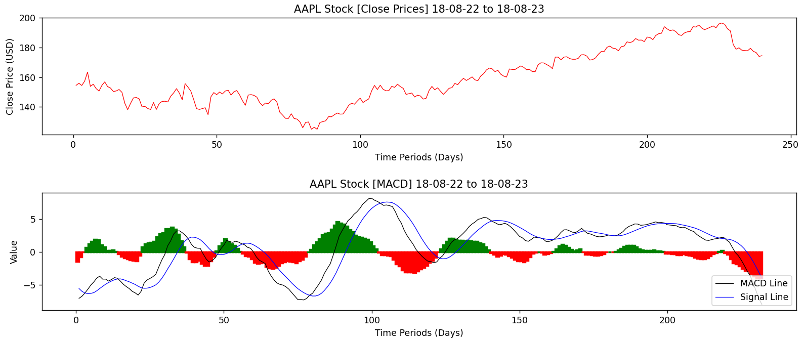
Source: Brandon Sandhu

We have two graphs, the above is the Apple closing stock prices and the bottom is the various components of the MACD indicator. Let us look into each component.

The most viable component in the bottom graph is the histogram values. Generally, the histogram goes negative and red when the stock is showing a negative trend and it goes positive and green when the stock is showing a positive trend.

. The histogram plot is useful for identifying trends in short intervals. The histogram also spreads more when the difference between the MACD and Signal Line is greater.

The next two components are the MACD line and the Signal line. The MACD line is coloured in black and is simply the difference between a fast and short EMA of the stocks closing prices. The Signal line in blue is smoother than the MACD since it is averaging out the MACD.

Trading Strategy

Now that we have some theory on two traditional indicators, let us discuss our unconventional trading strategy that we shall also implement in python. Let us define some technical terms before continuing.

We say we go long with a stock if we are buying the stock.

We short a stock if we are selling the stock.

The strategy is to go long if the %K and %D lines go below the 30 threshold on the Stochastic Oscillator and the MACD line and Signal lines are below -2. Similarly, we go short if the %K and %D lines go above the 70 threshold and both components of the MACD indicator are greater than 2. We can represent this trading strategy as follows:
IF %K < 30 AND %D < 30 AND MACD.L < -2 AND SIGNAL.L < -2 ==> BUY
IF %K > 70 AND %D > 70 AND MACD.L > 2 AND SIGNAL.L > 2 ==> SELL

This is all there is to it, this concludes our theory part let us now implement this practically using python as our choice of language.

Implementation in Python

Step 1: Importing our packages

This is arguably the most important step. Our primary packages are going to be pandas to work with data, NumPy to work with arrays such as using the np.diff function and Matplotlib to plot our graphs and the math module to make use of some more complex functions such as the math.floor function. We may also make use of the requests module to make API calls for live data.

Python Implementation:

    
        # Importing packages
        
        import pandas as pd
        import numpy as np
        import matplotlib.pyplot as plt
        import math

Step 2: Extracting stock data

For my examples above using the Apple stock, I made use of https://finance.yahoo.com/quote/AMZN/history/ which provides latest stock data and a timescale. It stores all the data in a CSV file which is crucial for when working with data using pandas. The file used in my examples is provided at the end of the article in a compressed zip folder. Alternatively you may use the requests module to make calls to an API which provides the same data but makes accessing live and more recent data much easier with a simple function call.

Python Implementation:

    
        # Read the CSV file
        amzn_data = pd.read_csv("AMZN.csv")
        
        close_prices = amzn_data[amzn_data.columns[4]]
        low_prices = amzn_data[amzn_data.columns[3]]
        high_prices = amzn_data[amzn_data.columns[2]]

Code Explanation:

The pd.read_csv command allows you to read the csv data into a DataFrame object. We use amzn_data.columns to call the columns of the data file and then read each column into their own respective variables namely close_prices, low_prices and high_prices respectively.

If you plan to use an API call to request the stock data then some cleaning up may be required since most APIs return data in JSON format hence you will be required to clear data up and turn it into a CSV format for pandas to read it into a pandas DataFrame. One could process the data in its raw form but this would become messy and in this field of programming clean code is a very crucial discipline especially when handling much more complicated indicators and computations.

Step 3: Stochastic Oscillator Calculation

In this step, we are going to calculate each of the components of the Stochastic Oscillator by the same methods and formulas as discussed above.

Python Implementation:

    
        # Stochastic Oscillator Calculation
        
        KValuePeriod = 14
        DValuePeriod = 3
        
        KValues = []
        for x in range(KValuePeriod, (len(close_prices) + 1)):
          LowOverPeriod = min(low_prices[x - KValuePeriod:x])
          HighOverPeriod = max(high_prices[x - KValuePeriod:x])
          KValues.append(100 * ((close_prices[x - 1] - LowOverPeriod) / (HighOverPeriod - LowOverPeriod)))
            
        DValues = []
        for x in range(DValuePeriod, (len(KValues) + 1)):
          SumOfPeriod = sum(KValues[x - DValuePeriod:x])
          DValues.append(SumOfPeriod / DValuePeriod)

Code Explanation:

The two variables KValuePeriod and DValuePeriod define the time ranges to go back into the past as discussed before. These are set to the conventional 14 and 3 respectively. We then iterate over the close_prices array but we begin at the KValuePeriod index so that we have enough data points to go back into the past. We then compute both the minimum and maximum of these data points and store these to the variables LowOverPeriod and HighOverPeriod respectively. We finally do the computation discussed before and append this to the KValues array which represents the %K line.

We perform a similar procedure to compute the %D line. We make use of the standard python sum, min and max functions.

Step 4: MACD Calculation

In this step, we are going to calculate all the components of the MACD indicator using our extracted Apple stock data.

    
        # MACD Calculation
        
        SlowLength = 26
        FastLength = 12
        SignalPeriod = 9
        
        SlowEMA = []
        for x in range(SlowLength, len(close_prices) + 1):
          SumOfPeriod = sum(close_prices[x - SlowLength:x])
          SlowEMA.append(SumOfPeriod / SlowLength)
        
        FastEMA = []
        for x in range(FastLength, (len(close_prices) + 1)):
          SumOfPeriod = sum(close_prices[x - FastLength:x])
          FastEMA.append(SumOfPeriod / FastLength)
        
        FastEMA = FastEMA[(len(FastEMA) - len(SlowEMA)):]
        
        MACD = []
        for x in range(0, len(FastEMA)):
          MACD.append(FastEMA[x] - SlowEMA[x])
        
        SignalLine = []
        for x in range(SignalPeriod, (len(MACD) + 1)):
          SumOfPeriod = sum(MACD[x - SignalPeriod:x])
          SignalLine.append(SumOfPeriod / SignalPeriod)
        
        MACD = MACD[(len(MACD) - len(SignalLine)):]
        Histogram = []
        for x in range(0, len(MACD)):
          Histogram.append(MACD[x] - SignalLine[x])

Code Explanation:

We again define the SlowLength and FastLength variables to be our slow and fast EMAs respectively. The SignalPeriod variable is the time period for our Signal line. We iterate over the stock prices shifted by the respective lengths so for the first stock we have sufficient data to go back into the past to compute its average. The average is computed using the python inbuilt sum function. The MACD is simply the difference between the two EMAs. The Signal line is averaging the MACD using the SignalPeriod variable as the time period. It is for this reason the Signal line is smoother than the MACD. Finally we take the difference between the Signal line and the MACD to be an indicator for the trend and store these values in the Histogram array.

Step 5: Creating the trading strategy

In this step, we are going to implement the Stochastic Oscillator and Moving Average Convergence/Divergence indicators to create our combined trading strategy.

Python Implementation:

    
    def Implement_STO_MACD_Strategy(close, k, d, macd, macd_signal):
      buy_price = []
      sell_price = []
      sto_macd_signal = []
      signal = 0
    
      minIndex = min([len(close), len(k), len(d), len(macd), len(macd_signal)])
      k = k[(len(k) - minIndex):]
      d = d[(len(d) - minIndex):]
      close = list(close[(len(close) - minIndex):])
      macd = macd[(len(macd) - minIndex):]
      macd_signal = macd_signal[(len(macd_signal) - minIndex):]

      for x in range(len(close)):
        if k[x] < 30 and d[x] < 30 and macd[x] < -2 and macd_signal[x] < -2:
          if signal != 1:
            buy_price.append(close[x])
            sell_price.append(np.nan)
            signal = 1
            sto_macd_signal.append(signal)
          else:
            buy_price.append(np.nan)
            sell_price.append(np.nan)
            sto_macd_signal.append(0)
        elif k[x] > 70 and d[x] > 70 and macd[x] > 2 and macd_signal[x] > 2:
          if signal != -1 and signal != 0:
            buy_price.append(np.nan)
            sell_price.append(close[x])
            signal = -1
            sto_macd_signal.append(signal)
          else:
            buy_price.append(np.nan)
            sell_price.append(np.nan)
            sto_macd_signal.append(0)
        else:
          buy_price.append(np.nan)
          sell_price.append(np.nan)
          sto_macd_signal.append(0)
      return buy_price, sell_price, sto_macd_signal, close

Code Explanation:

We begin by defining a function Implement_STO_MACD_Strategy which takes parameters close our stock close prices, k our %K line, d our %D line, macd our MACD line and macd_signal our Signal line.

Inside the function we create three empty arrays buy_price, sell_price and sto_macd_signal in which values will be appended whilst creating our trading strategy.

After initialising our variables, we use a for loop to create our trading strategy based on our two indicators. Inside the for loop, if the conditions for buying a stock are satisfied then we append the buying price into buy_price and 1 is appended into sto_macd_signal which tells us to buy the stock. Similarly, if the conditions to sell a stock are satisfied then we append the selling price into sell_price and -1 is appended into sto_macd_signal which tells us to sell the stock. Finally, we return the signal array, sto_macd_signal along with its buying and selling prices at the appropriate index positions. We additionally also return the truncated stock close prices so that the dimensions of all these arrays are equal.

Step 6: Backtesting

Backtesting is the process of testing our trading strategy on given stock data to see how well it performs. For our case we will implement a backtesting process on our Stochastic Oscillator and MACD trading strategy using the Apple stock.

Python Implementation:

    
        InitialInvestment = 100000
        NumberOfStocks = 0

        for x in range(len(sto_macd_signal)):
          if (sto_macd_signal[x] == 1):
            NumberOfStocks = math.floor(InitialInvestment / buy_price[x])
            InitialInvestment -= buy_price[x]*NumberOfStocks
          elif (sto_macd_signal[x] == -1):
            InitialInvestment += sell_price[x]*NumberOfStocks
            NumberOfStocks = 0
        print("Return: " + str(round(InitialInvestment, 2)))

Code Explanation:

We set InitialInvestment to be 100000, our initial investment. Then we iterate through our signals array sto_macd_signal and if the signal is 1 then we buy the stock at the given buy price supplied in the buy_price array. Similarly, when the signal is -1 we sell the stock at the given sell price supplied in the sell_price array. This will complete our trading strategy on our investment and print our total return.

Conclusion

After going through both the theory and coding parts, we have successfully learned what the Stochastic Oscillator and the Moving Average Convergence/Divergence is. We have created a trading strategy involving both indicators one which describes the state of the market as to whether it is overbought or oversold and one which gives us the trend of the stock in a short time interval. We expect the stock to be high in value when it is overbought and combining this with an increasing trend from the Moving Average Convergence/Divergence indicator we can make a decision when to sell a stock. By similar means we can make a decision of when to buy a stock.

The main take away from this article is that of the application of programming in financial mathematics with a key example being the stock market. We can most certainly conclude that in order to hold a strong edge on the market, it is essential to master the art of programming and being able to apply this to process very large amounts of data to provide us insight into the hidden trends within stock data.

The source files and data files used in this article can be found here

Thank you for reading this article, for any questions or queries I can be emailed at me@brandonsandhu.com